Two Kelly betting rules: one of which I might actually remember

I was having a conversation the other day involving proportional betting and the Kelly criteria, and was embarrassed that I couldn't remember of the top of my head what some of the numbers came out to be. So I decided to try to make this really simple for myself by supplying two rules. The first applies to betting on an even money favorite. The second applies to betting on longshots. Both assume you wish to maximize the log of your wealth.

RULE 1: If "heads" is ten percent more likely than usual, bet ten percent of your wealth.

Here's a plot of \(E[log(1+fX)]\) where \(X\) is a binary random variable taking value \(1\) or \(-1\) with probability \(0.55\) and \(0.45\) respectively. The x-axis shows \(f\), the fraction of one's wealth one decides to put on the coin flip.

Percentage of one's wealth to wager on a coin flip with p=0.55

The y-axis can be interpreted as the average return, if we assume we get paid even money even though we know the true probability is different. Clearly we want to bet about ten percent of our wealth to maximize this.

But is the scale wrong? Since we have a ten percent edge we should, on average, be making ten percent of ten percent return, or one percent return, right?

Well no. You only get half that. If you want to remember why you only get half a percent, not a one percent return, notice that you are approximately maximizing a linear function (the return you expect, not taking into account the \(log\)) subject to a quadratic penalty (the concavity of \(log\)). To be more precise we observe the expansion around  \(f=0\) of
\begin{equation}
  E[\log(1+X)]  = 0.55 \log(1+f) + 0.45 \log(1-f)
\end{equation}
which is given by
\begin{equation}
0.55 \log(1+f) + 0.45 \log(1-f)  = \overbrace{0.1 f}^{naive} - \overbrace{\frac{1}{2} f^2}^{concavity} + O(f^3)
\end{equation}
The next two terms are \(+ \frac{1}{30} f^3 - \frac{1}{4} f^4\) incidentally. But as might be surmised from the plot we are pretty close to a parabola. The marginal return goes to zero just as the parabolic term starts to match the linear one (i.e. its rate) and the absolute return goes all the way to zero when the parabolic term wipes out the linear one completely. So it must be that we optimize half way down, as it were.

Another way to come at this is that the fraction of wealth you should invest is simply \(p-q\). That's surprising at first. But since \(E[log(1+X)]  = p \log(1+f) + q \log(1-f) \) in general we note that
\begin{equation}
     \frac{\partial}{\partial f} E[\log(1+X)]  = \frac{p}{1+f} - \frac{q}{1-f}
\end{equation}
which is zero for
\begin{equation}
        f = p - q
\end{equation}
Incidentally your return grows slightly faster than the square of your edge. As the amount we bet is linear in the edge, we'd expect the return to grow quadratically as we vary \(p\), more or less. And not forgetting the factor of one half it ought to be half the square of our edge. In fact it grows slightly faster, as can be seen by substituting the optimal \(f= p-q\) back into the return equation.

Average return for an even money coin flip. 

The actual return is the red line. The quadratic approximation is the blue. Not that the percentage edge is \(2(p-0.5)\), not \(p-0.5\).

So much for betting on the favourite, as it were, but what about longshots? The the math doesn't change but our intuition might. Instead of fixing the outcome at even money and varying the true probabilities of an outcome, let's instead fix the true probability at \( p = 0.01 \) and vary the odds we receive. All being fair we should receive $100 back, including our stake, for every $1 bet. We'll assume instead we get a payout of \(\alpha\) times the fair payout.  Then we maximize
\begin{equation}
  E[\log(1+X)]  = p \log\left(1+ f \alpha \left( \frac{1}{p}-1\right) \right) + (1-p) \log(1-f )
\end{equation}
This brings us the the second easy to remember betting rule.

RULE 2. If a longshot's odds are ten percent better than they should be, bet to win ten percent of your wealth. 

Now I know what you are thinking: why do we need rule #1 if we have rule #2? Well you probably don't, actually, but evidently I might because I have managed to forget rule #2 in the past. We'll call it a senility hedge.

But rule 2 the rule is quite reasonable on a larger domain - though eventually it too breaks down. If you can get ridiculously good odds on a longshot (let's say ten times the fair odds) don't go absolutely nuts. Only bet the amount that would double your wealth if the odds were fair. Diminishing returns set in if you are set to win so much that the concavity of \(log\) kills the fun. You can see that in the picture below.

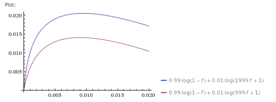Average return on a 100/1 horse when we are offered 1000/1 and 2000/1 respectively. 

Notice that we bet only marginally more if we get 20 times the fair odds versus 10 times. We do win twice as much, however.